
“How can we improve the conversion rates of incoming leads?”
“How do we improve sales team’s efficiency?”
“Which is the best medium to target leads?”
These are some questions that sales managers are commonly asked. The best answers to such questions lies with data. This is why scoring incoming leads based on various data points can help in effective targeting.
At Razorpay, we have tried two common approaches to arrive at a lead score.
1) Heuristics based scoring
This approach involves providing weightage to various important factors based on intuition and on the lead score. The leads in the high scoring bucket are reached out using calls, the ones with medium score are reached out using SMS, and the remaining in low scoring buckets could be reached out via emails. The thresholds of these buckets could be decided based upon the team’s capacity for handling calls.
For instance, let’s suppose an inbound sales team of 5 members can call a maximum of 100 leads a day out of 500. Then the top 20% leads could be classified as high quality buckets and the remaining could be placed under medium and low-quality buckets. This method is used when an organisation is in its early stages and there is insufficient historical data to learn from.
2) Machine Learning based leads scoring
This approach requires leveraging historical data to identify the most significant features that result in lead conversion, computing features weightage, and building a predictive model to score new leads.
This type of method is applied when there is sufficient sample size available. As a thumb rule, the minimum sample size for the binary logistic regression model could be determined using the basic formula, n = 100 + 50i, where i is the number of features used in the statistical model. For instance, if we have 5 features, then the minimum sample size required to create the model=350.
The first approach is pretty simple and straightforward, so a detailed explanation of the same is skipped. Here, the implementation of the second approach to create a leads scorecard is discussed in detail. The scorecard is very easy to interpret and could be easily understood by people with no technical background. A sample leads scorecard with two features is shown below.
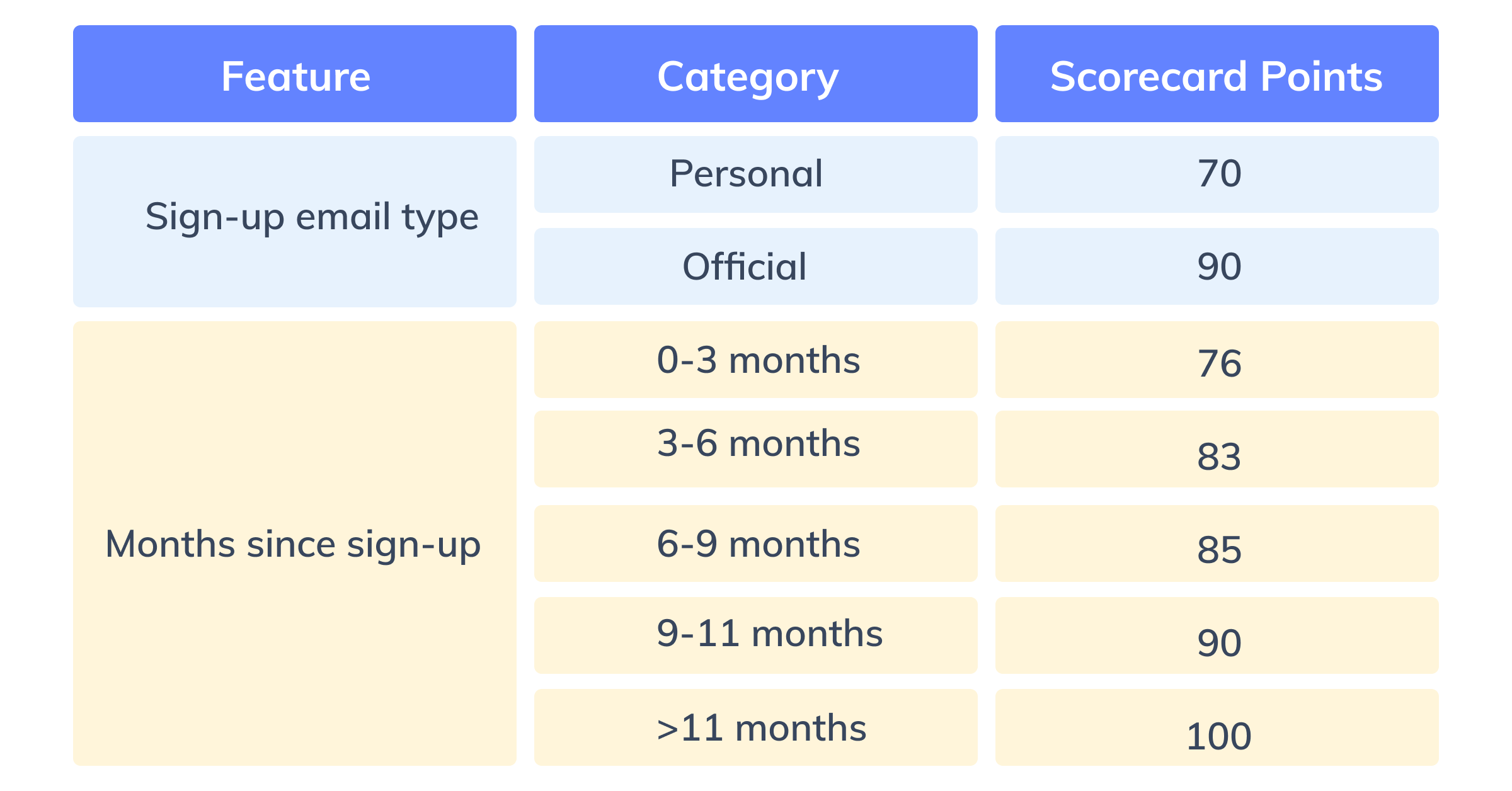 Figure 1: Sample scorecard with two features
The problem statement
There are a lot of customers who sign up on the Razorpay website expressing their interest to become partners. However, the volumes of signups and limited team size makes it difficult for the sales team to get in touch with all the leads. This is where the lead scorecard comes to the rescue. There are two main parts in building the scorecard:
- Developing a statistical model
- Applying the statistical model to compute the lead score for a partner merchants
Statistical model
Building a statistical model involves data collection, exploration, transformation, feature selection, model training, and model testing.
Step 1: Data Collection
We gathered historical data of 10,000+ partners to study the influence of various factors on their conversion. Shown below are the first set of all the features, called independent variables, and the outcome variables.
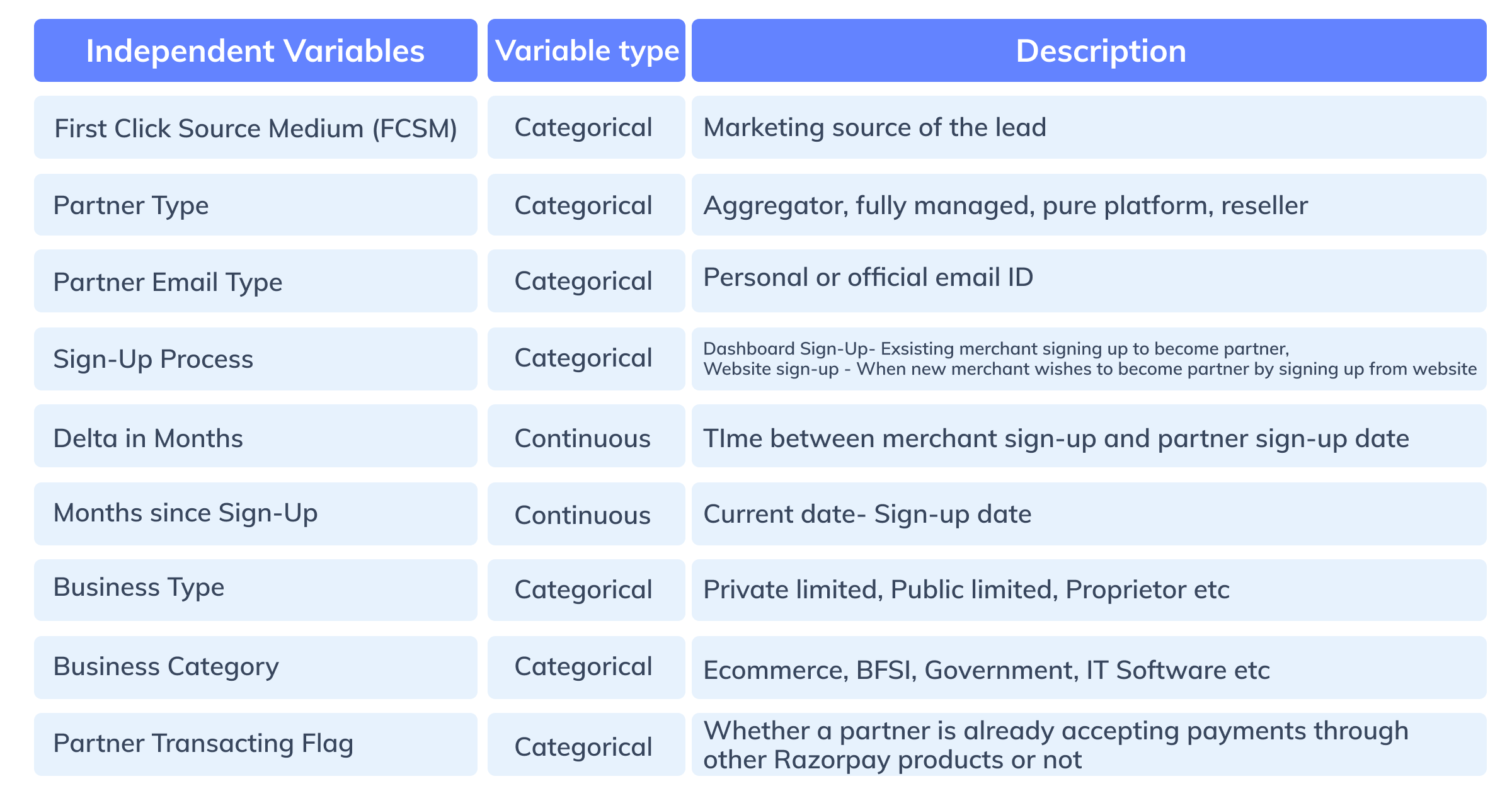 Figure 2: Independent features for the data model
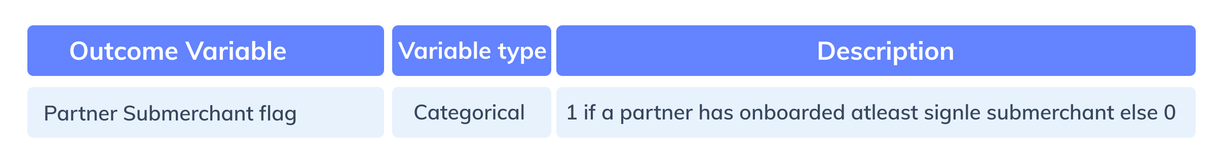 Figure 3: Target feature for the data model
In the blog, the partner merchants who have referred and on-boarded at least one sub-merchant are referred to as “Good partners” and the rest are referred as “Bad partners”.
The dataset is divided into training and test – training for learning from the historical data, and testing for evaluating model accuracy metrics.
Step 2: Data Exploration
Data exploration involves a univariate and bivariate analysis of various independent features to understand basic trends in data.
The univariate analysis involves only one variable for summarising the data. Histograms, box plots, etc are some of the most common graphs for performing univariate analysis of continuous features.
The bivariate analysis involves more than one variable for determining empirical relationships between them. It could be descriptive as well as inferential. The bivariate analysis could be done between two continuous or categorical features or one continuous and one categorical feature. Stacked bar charts, correlation plots, etc are some of the generally used graphs for bivariate analysis.
Step 3: Data Transformation
This step involves transforming all the features using the weights of evidence(WOE) method. All the categorical variables can be directly transformed, whereas continuous features (like Delta in months, Months since signup) are bucketed before WOE imputation. The buckets could be created based on the percentile approach or business intuition.
WOE provides the weights for each of the categories of features, based on the distribution of good partners and bad partners.
Information value(IV) is a useful method for measuring the predictive strength of features and for selecting significant features for the model. Figure 4: Mathematical formula for WOE and IV
The WOE and IV calculations for each category of one of the continuous features (Month since signup) is shown below.
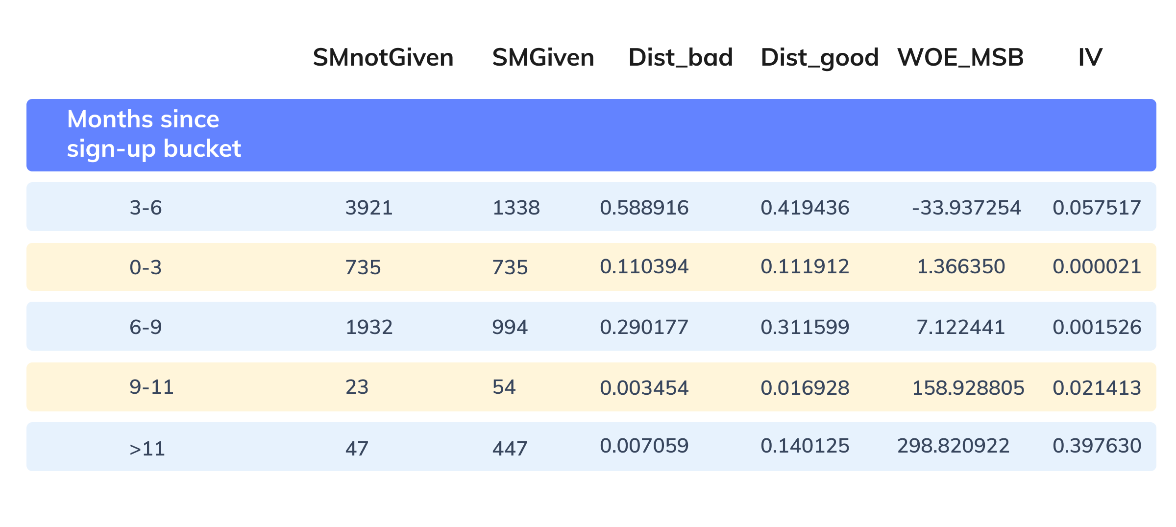 Figure 5: WOE and IV computation for a continuous feature (Features analysis reports)
Where:
- SMnotGiven denotes the count of bad partners
- SMGiven denotes the count of good partners
- dist_bad denotes the proportion of bad partners amongst all the bad partners
- dist_good denotes the proportion of good partners amongst all the good partners
- WOE_MSB denotes weights of evidence (WOE) for months since the signup feature
If the distribution of good merchants is greater than the bad merchants, WOE is positive, else negative or zero. The higher the WOE, the more weightage of a particular category, and the higher would be the final category score of a feature.
All the raw data inputs are finally substituted with their corresponding WOE values.
Step 4: Feature selection
Before running a statistical model, it is vital to select only important features. The Information Value(IV) corresponding to each of the features is computed and only features with IV between 0.02 to 0.5 are considered. That’s because features with IV less than 0.02 are insignificant for the model and greater than 0.5 can result in model overfitting.
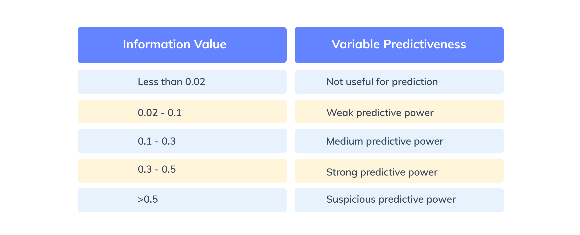 Figure 6:Nadeem Siddiqi (2006) interpretation of IV Values
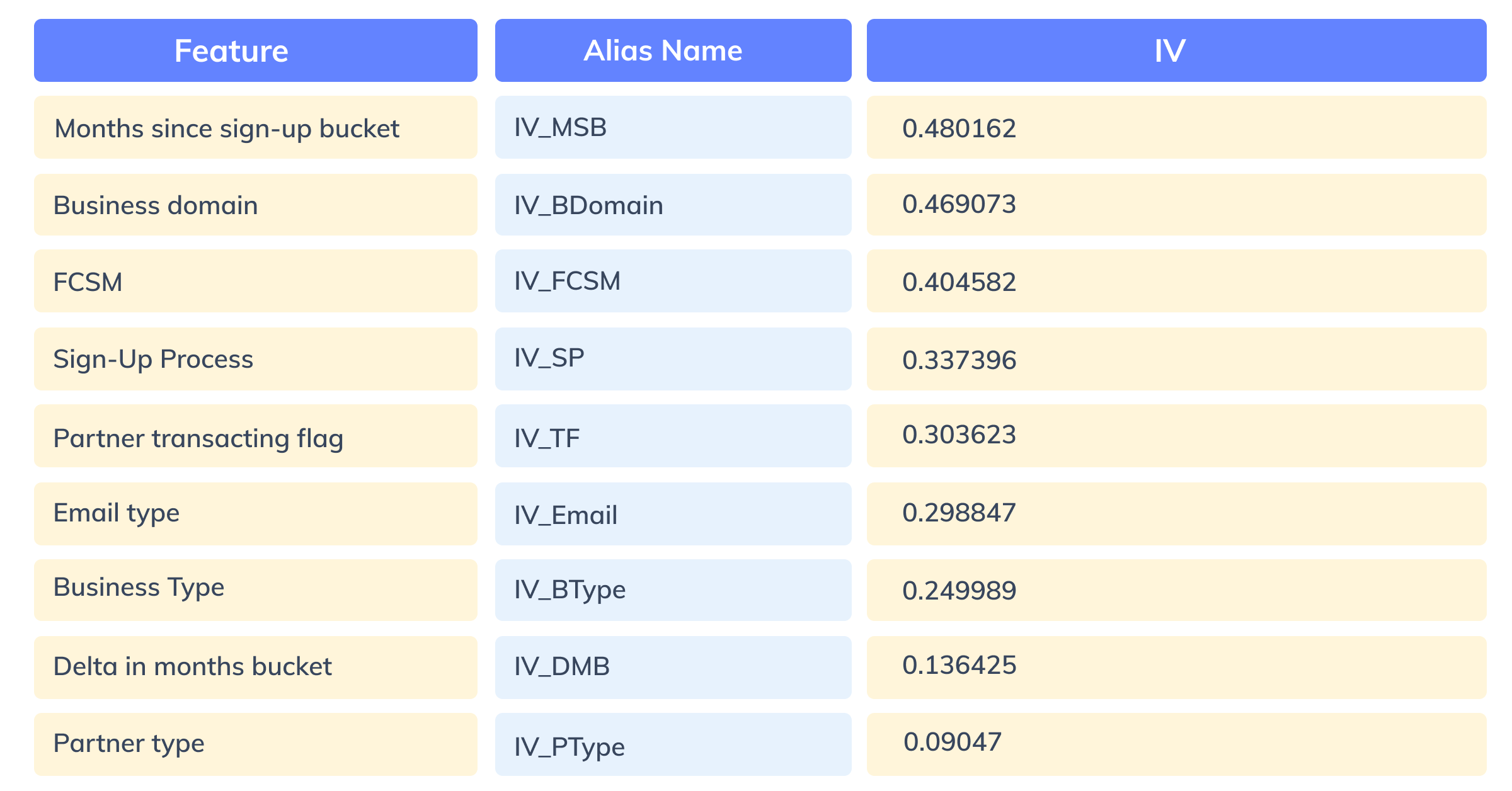 Figure 7: IV Values for all the important features
Step 5: Model training
Now we fit our logistic regression model with WOE values as input features and a target categorical variable.
For scaling the model into a scorecard, we consider WOE values derived in step 3 and coefficients derived by training the logistic regression model.
The score for each category feature can be computed with the formula:
Score = (β×WoE+ α/n)×Factor + Offset/n
Where:
- β — logistic regression coefficient for the feature
- α — logistic regression intercept
- WoE — Weight of Evidence value for the given category in a feature
- n — number of features included in the model
- Factor, Offset — scaling parameter
The first four parameters have already been calculated in the previous part. The following formulas are used for calculating factor and offset.
- Factor = pdo/Ln(2)
- Offset = Score — (Factor × ln(Odds))
Here, pdo means points to double the odds and the bad rate has been already calculated in the features analysis reports above.
If a scorecard has the base odds of 2:1 at 600 points and the pdo of 20 (odds to double every 20 points), the factor and offset would be:
Factor = 20/Ln(2) = 28.85
Offset = 600- 28.85 × Ln (2) = 487.14
The score derived for one of the features is shown below.
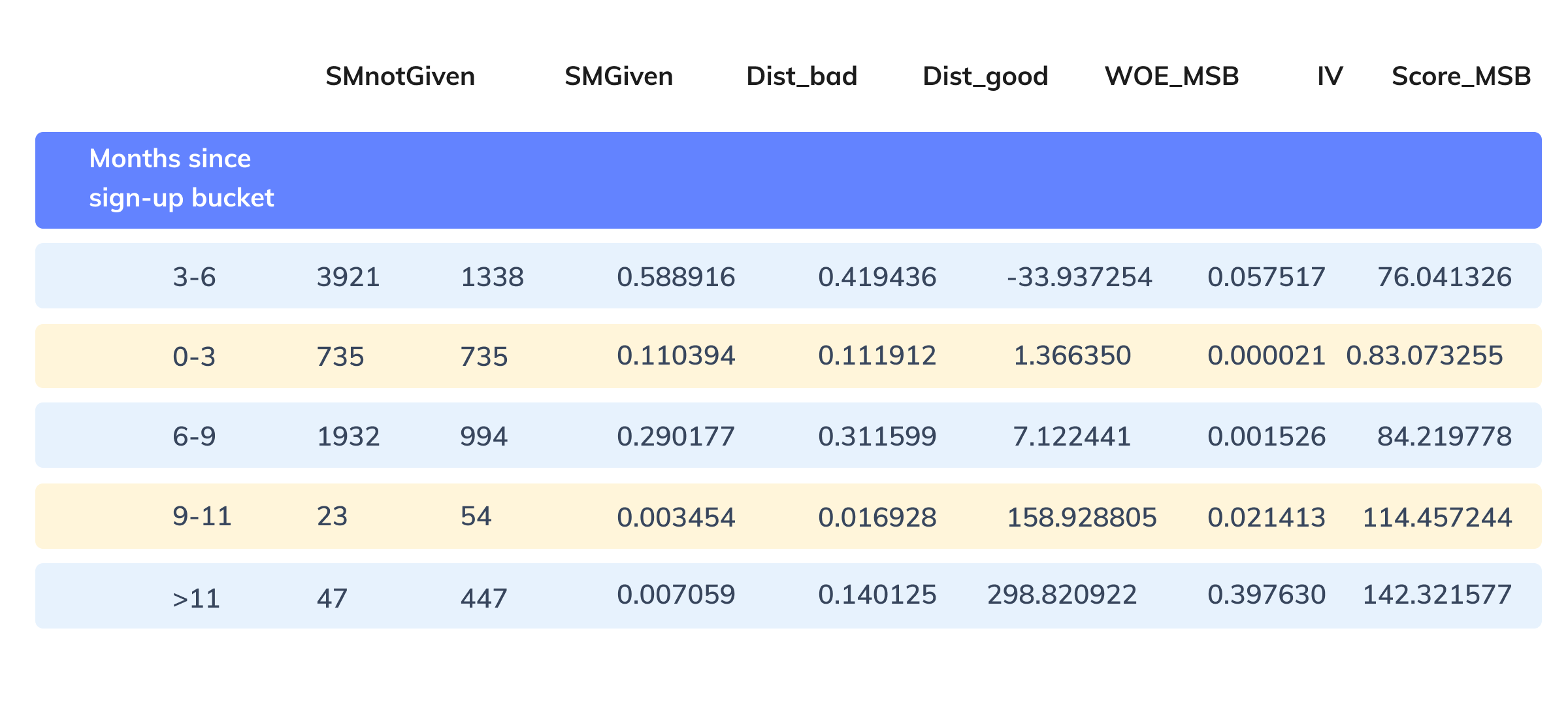 Figure 8: Category wise lead scores for Months since the signup feature
The scores are derived similarly for all the features to create a lead scorecard with 7 features.
Note: The choice of the scaling parameters does not affect the predictive power of the scorecard.
Step 5: Model Testing
The model is tested on unseen partner leads and the accuracy of the model on the test dataset comes around ~73%. False positives (78 merchants) are a bigger concern than False Negatives as that would lead to opportunity loss for the sales team.
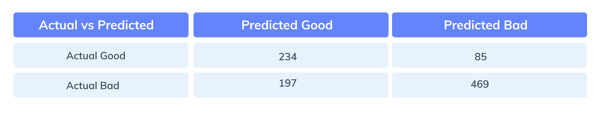 Figure 9: Confusion matrix of the test dataset
Where:
Predicted_Good is defined on threshold score=580 i.e if the predicted lead score >580, then the partner test lead is classified as 1 or else as 0. The optimal threshold cutoff is decided based on the evaluation of precision and recall metrics across some fixed threshold scenarios, and the sales team capacity.
Recall and Precision are two important metrics for imbalanced classification models. Recall indicates that out of the total actual good leads(319 partners), what percentage of leads are classified correctly. Precision refers to the percentage of correct classifications out of the total predicted good leads(413 partners).
In mathematical terms,
Recall=(TP) /(TP+FN)
Precision=(TP)/(TP+FP)
Where:
TP= True Positive, FP=False Positive, TN=True Negative, FN= False Negative
Lowering the threshold increases the recall and merchant base for human-based targeting, thereby increasing sales team effort. On the other hand, increasing the threshold, decreases the recall, increases the precision, and may result in opportunity loss for the sales team. The table below demonstrates the same.
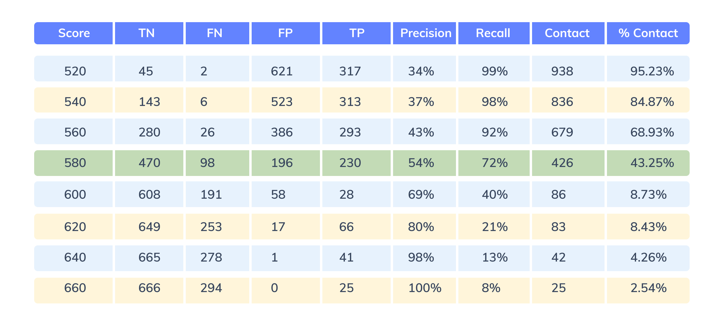 Figure 10: Determining the optimal threshold score for classification
At threshold 580, precision=54%, recall=72%, and % merchants to be targeted via human-based targeting out of the total merchants is ~43%. Considering 580 satisfies all three criteria, it is considered to be the optimal threshold cutoff for classifying good and bad partners.
The model consumption
For deriving the lead score for a merchant, all the individual feature scores based on each of the categories are added up.
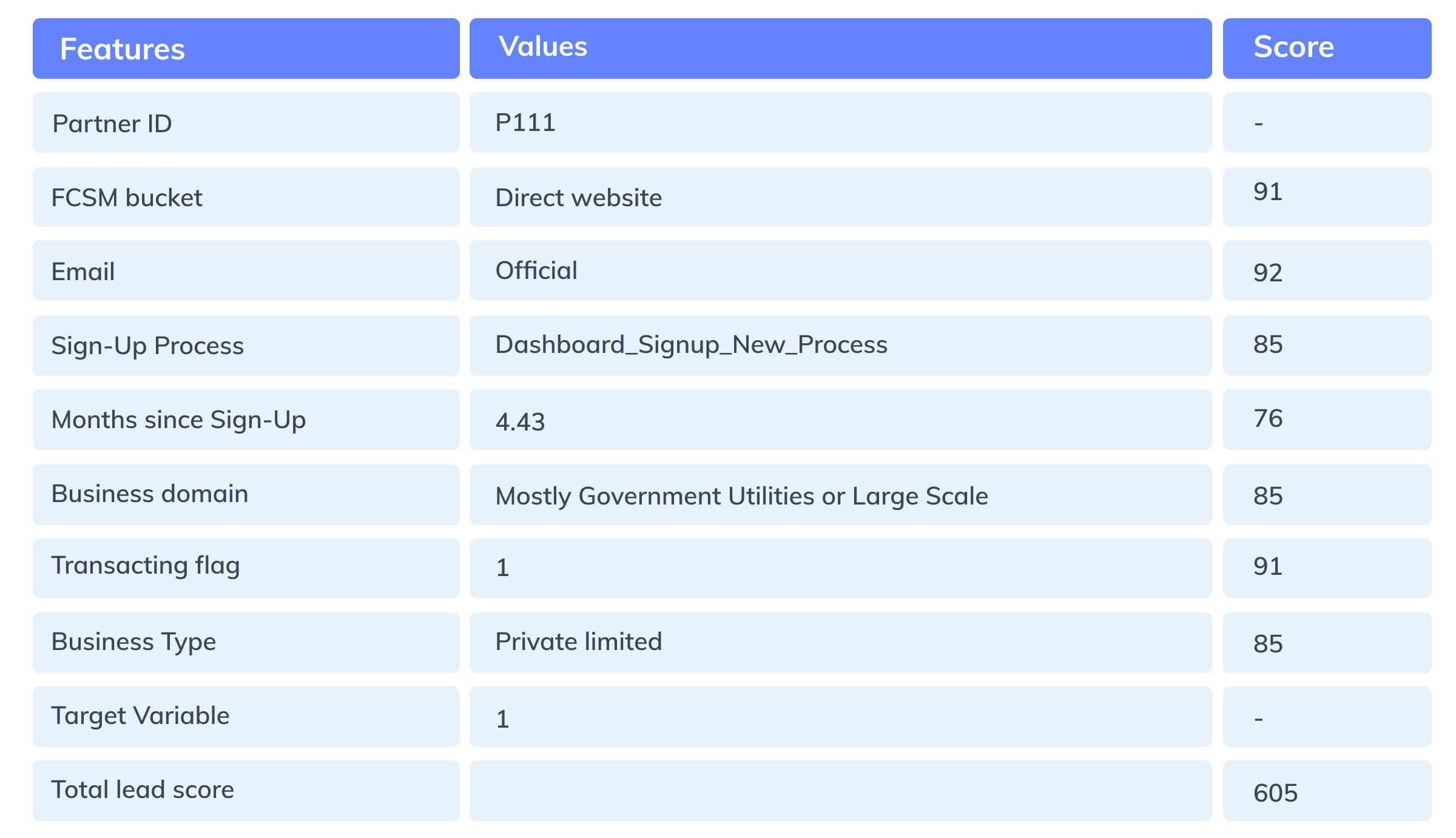 Figure 11: Sample lead scorecard for a partner merchant
The lead scoring rules are finally integrated with CRM tools like Salesforce. All the leads piped to a specific queue are scored. The leads above the threshold score, also called high-quality leads(HQLs), are targeted daily using calls and the rest are targeted with personalised and generic emails.
The business impact
To understand the effectiveness of the model, data is analysed pre and post implementation of the model.
- The leads gestation period i.e time taken by lead to become live on Razorpay platform has reduced by approximately by a month
- The effort of the sales team has gone down drastically by 70% (~1000+ man-hours) to achieve the same level of conversion rates
- There has been a 50% increase in monthly GMV, indicating more time spent by the sales crew on high-quality leads
And that is how machine learning based lead scoring has helped us scale.


